Along with colleagues from Ohio State University, we took a look recently at data from a lot of corn plant population trials in both Ohio and Illinois to see if we could come up with estimates of the value of variable-rate corn planting. This work was published in Agronomy Journal (reference is at the end of this article) and my OSU colleagues also put the findings in an Extension fact sheet, available here.

It’s not so difficult to do seeding rate trials with today’s planting equipment and yield monitors, and it’s even possible to do several of these within a field in order to get an idea of how much responses vary within the field. The difficulty is that responses within parts of a field are not consistent across years: they are often more dependent on weather conditions than on soil zone or soil type. As an example, yields in recent years with wet spring weather have often been higher on sloping parts of fields than in the flatter, higher-organic matter soil where we would normally expect more yield, and so be inclined to drop more seeds.

One solution to this problem is to do a simulation, using existing data from a number of population trials over sites and years to get an idea of how much we might expect population responses to vary within a field with different soils and in different years. To do this, we turned the yields from each individual trial into “return to seed” (RTS) data, by taking yield times the corn price at each planting rate and subtracting the seeding rate times the cost of seed. For this exercise, we used a corn price of $3.75 per bushel and seed cost of $3.00 per thousand. So if the yield in a trial was 220 bushels per acre at a seeding rate of 36,000, the return to seed at that population was 220 x $3.75 – 36 x $3.00 = $717 per acre.

The response of corn yield to plant population/seeding rate (we use these interchangeably here; with the precision planter we use for plots, they are nearly identical in most cases) usually takes one of two shapes: 1) yield increases as a curve up to a certain population, then levels off at higher populations—we call this a “quadratic+plateau” (Q+P) response; or 2) yield increases as a curve up to a certain population, then declines at higher populations—this is a “quadratic” (Q) response. When yield data are converted to RTS data, a QP response rises to a maximum, then declines as a straight line, with loss at higher population as seed cost increases but yield doesn’t. The data from a Q response, though, shows RTS rising up to its maximum, then declining at higher populations at the same rate as it increased, weighed down both by higher seed costs and loss of yield. Curves from two Illinois trials that illustrate these two responses are shown in Figure 1.

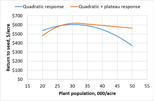
Figure 1. Examples from Illinois trials with return to seed (RTS) data fit by a quadratic+plateau function compared to a quadratic curve. The population that maximizes RTS is similar (between 30 and 31 thousand) for both curves, but the dollar penalty for having population too high is much larger when the response is quadratic.

The maximum point on either a Q or QP curve plotted as RTS is what we call the “optimum” seeding rate, or the one that produced the maximum economic return. Using the prices given above, adding the last 1,000 seeds needs to increase yield by $3.00 ÷ $3.75 = 0.8 bushels per acre in order to pay for itself. We used data from 32 Illinois trials in this work, and the RTS curves from each trial are shown in Figure 2. Nine of these trials showed a Q response, and 23 showed a QP response. All of the Q responses show a curved decline at higher populations, and the QP ones decline as straight lines to the right of their maximum points.

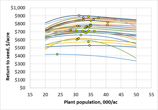
Figure 2. Return to seed (RTS) response to corn plant population in 32 Illinois trials conducted between 2010 and 2016. The yellow circles mark the high point of each curve, which is the “best” population for that trial.

We averaged the RTS values at each population across all 32 Illinois sites, and found that the maximum RTS ($740.05, from a yield of 224.05 bushels per acre) occurred at a population of 33,377 plants per acre. We’ll consider that the best uniform seeding rate (USR) in this exercise. Across trials, the population at the maximum RTS (yellow circles in Figure 2) ranged from 23,942 to 40,609, and averaged 33,399 plants per acre, or 22 plants per acre more than the 33,377 in the “uniform” seeding rate. The maximum RTS values ranged from $420.32 to $905.21 per acre, and averaged $742.89 per acre.

Now let’s pretend that each trial represents a 2.5-acre part of an 80-acre field. The “best” population in each block is the population that produces the maximum RTS in that block (trial): we can’t really know what that is beforehand, but here we’re using that range (23,900 to 40,600) as one that might apply in a variable field, and we’re pretending that we know just which block gets which seeding rate. As noted above, using “VRT” meant planting an average of 33,399 seeds per acre, and produced an average yield of 224.82 bushels per acre, for an overall RTS of $742.89 per acre.

The USR of 33,377 per acre was higher than the VRT seeding rate in about half the blocks and lower in the other half; the USR is not (by definition) exactly the best seeding rate for any one block. In other words, a uniform seeding rate across the field reduces the RTS in every part of the field. Doesn’t that mean that VRT is superior to USR every time? Yes, but the issue (in addition to the larger issue of knowing how to set VRT rates) is how much added return we can get from VRT. With Illinois data, the improvement in RTS in a block ranged from less than one cent to $11.60 per acre; in only half of the blocks did VRT produce more than $1.00 greater RTS than USR. Overall, VRT produced $2.84 more than USR: $2.90 from getting 0.7 more bushels with VRT, and subtracting the 22 more seeds ($0.06/acre) needed for VRT.

Results in Ohio were quite different from those in Illinois. More than 75% of the 93 Ohio trials showed a quadratic response to population. Quadratic responses result from having high populations high enough to decease yield, and this is more common in less-productive soils, under poor weather conditions, or where the maximum population is set very high. Because quadratic responses mean large losses in RTS at high populations, VRT, by avoiding such penalties, provides more of an advantage over USR when responses are mostly quadratic. Across the Ohio trials, the USR seeding rate was 32,721 per acre and the average VRT rate was 592 seed lower, at 32,129 seeds per acre. The yield with VRT was 205.5, or 2.9 bushels per acre higher than with USR, and the RTS with VRT was $12.53 higher than with USR: $10.76 from higher yield and $1.77 from the lower seeding rate. This may signal that VRT might have more promise in forest-derived soils (which are more common in Ohio), but that needs to be confirmed by running trials on such soils in Illinois.

So, VRT or not?

With today’s equipment, VRT can be done with little cost, depending on how much we pay for a planting map. So why not use it in most fields, even if returns are modest? There are fields where it makes a lot of sense, such as irrigated fields with unirrigated corners, where dropping the population by a lot may often increase yields in very light soils. There are also fields with soil types ranging from clay loam to sandy loam, where adjusting populations by soil type might make sense. It’s not always clear how such adjustments should be made, but any part of the field that tends to show drought stress (this could be on light or heavy soils) may benefit from somewhat lower population. Population should probably never be set so low that yields will take a hit if the weather turns favorable, though: a yield map from a year with above-average yields is a better guide to this than one from years when yields are below average. Most hybrids produce good yields at populations above 28,000 or so, and it is usually counter-productive to set the lowest VRT seeding rates to less than 30,000 seeds in most unirrigated fields, at least ones without very light soils.

What about VRT for prairie soils with only modest differences in soil productivity, and where yields maps in good years show good uniformity? [Be careful when comparing yield maps—some mapping programs assign colors after breaking yields into a fixed number of segments, so good yields with less variability might produce maps as “colorful” as average or lower yields with a lot of variability.] Then, do VRT by setting the lowest populations close to what you might use if you were doing uniform seeding, unless uniform seeding rates often exceed 35,000, in which case maybe 32 to 34 thousand might be better for lower-yielding areas. And go up from there, keeping in mind that raising seeding rates above 40,000 is unlikely to increase yield. Yield loss from having seeding rates too high is not very common, but in 2018, three of our six population trials showed yield declines from raising the population from 42 to 48 thousand, and averaged over all six trials, we lost 13 bushels—from 251 to 238—from this increase in population.

As with other aspects of managing today’s hybrids, using VRT is unlikely to show large increase in yields or saving of seed, and so we should avoid adding costs or using “high and higher” seeding rates because we’ve heard that high yields require high populations. Across the six trials we did in 2018, 35,800 maximized yield at 252 bushels per acre, but the average optimum population was 32,600, which produced an average yield of 251. Although this population is a few thousand less than we’ve sometimes found in trials, it’s likely that planting 35 or 36,000 per acre uniformly across less-variable fields will perform about as well as VRT, however we choose to do it.